Categories
Prefer INDEX and MATCH over VLOOKUP
The combination of INDEX and MATCH, as well as the VLOOKUP function are well known methods for search in Excel. To our great frustration, the latter is used a lot more often, while the combination of INDEX and MATCH is less error prone and a lot more efficient.
VLOOKUP
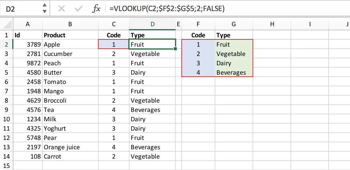
With VLOOKUP you search for the value in a certain column of a worksheet based on a selected value in the first column of the same table. This may sound a little complicated but essentially a set value is located in column one, and the matching value in column two is retrieved. The format is =VLOOKUP(C2; $F$2:$G$5;2; FALSE), where C2 is a reference to the value you are looking for in the first column, F2: G5 is the table you are searching in (the 2 means that you are looking for a result in the 2nd column of the table) and FALSE means that you want to search exactly (and not approximately).

MATCH
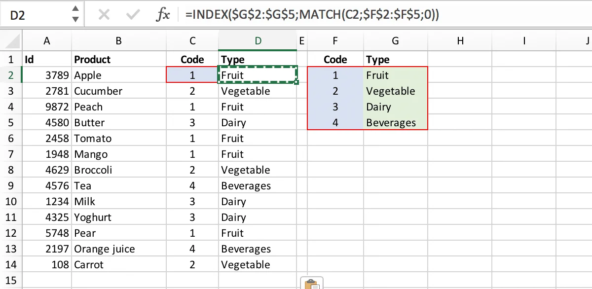
On the other hand, the MATCH function determines where a certain value occurs in the range. The format is =MATCH(C2;$F$2:$F$5;0). C2 is again the value you are looking for. F2: F5 is the range in which you are searching, the 0 means that you want to do an exact search.
INDEX
With the INDEX function, you can retrieve a certain value from a column. The certain value is often determined by a MATCH. The format is INDEX ($G$2: $G$5; X) in which G2: G5 is the row from which you need the Xth (the MATCH) value.

Often INDEX and MATCH are put together in a cell and then you get =INDEX (G2: G5; MATCH (C2; F2: F5;0)).
Prefer INDEX and MATCH!
Ay, it takes two paragraphs to explain the INDEX and MATCH and only one for VLOOKUP. Do you think it’s crazy that VLOOKUP is more popular? Well don’t look at it in this way! Instead, compare it to camping which really is much nicer with an inner and an outer tent. Even if takes a little longer to set up than a single roof tent, most people realize that it’s the best solution and that the result is worth the time. Take that effort! Here’s why it’s worth it:
1) The numeric reference (2, in the example) indicating the column from which the VLOOKUP must obtain a result is not flexible. If somebody ever inserts a column into the table – and this happens very often – the function no longer works, because it continues to take something from the third column while it should now be taking from the fourth one. You might think of adjusting the column number in the function, but think about the future user!
2) The necessary value “FALSE” is very often forgotten in VLOOKUP, if it is omitted or replaced by TRUE, the function “approximately” searches in a very special way, which is hardly ever needed/intended. In the MATCH function a value for exact search must also be entered (0), but for some reason it is less often forgotten.
3) For large tables and long chains of references, the INDEX and MATCH function can be much faster than the VLOOKUP. Especially if you need to find something several times based on the same match. In that case you can create a separate column for the MATCH and refer to that column in several INDEX formulas. Many users forget this, even if they are familiar with the INDEX and MATCH feature, but it makes the spreadsheet much more efficient.
Read more about the practical application of INDEX & MATCH in the article:
How can PerfectXL help?
What can PerfectXL Risk Finder do for you in this scenario? Well one of the things the PerfectXL engine searches for is Approximate Lookup. It searches for VLOOKUP (or HLOOKUP) functions with TRUE as last variable or cases where the final variable is omitted. This almost invariably goes wrong, so we draw the user’s attention to these instances.
Screenshot
In short, it takes some getting used to, but do it anyway: use the INDEX and MATCH!
