Categories
How to use HLOOKUP in Excel
HLOOKUP is a function that makes Excel search for a certain value in a row (the so called ‘table array’), in order to return a value from a different row in the same column. HLOOKUP stands for ‘Horizontal Lookup’.
About the HLOOKUP function
A HLOOKUP function in Excel exists of 4 components:
- The value you want to look up;
- The range in which you want to find the value and the return value;
- The number of the row within your defined range, that contains the return value;
- 0 or FALSE for an exact match with the value your are looking for; 1 or TRUE for an approximate match.
Syntax: HLOOKUP([value], [range], [row number], [false or true])
HLOOKUP Example
In our example we show how many pieces of fruits are sold per day in the first week of May. We want to find out how many oranges were sold each day of the week.
First, select a cell in which you want to publish the sold amount of oranges. We start with ‘Day 1’:
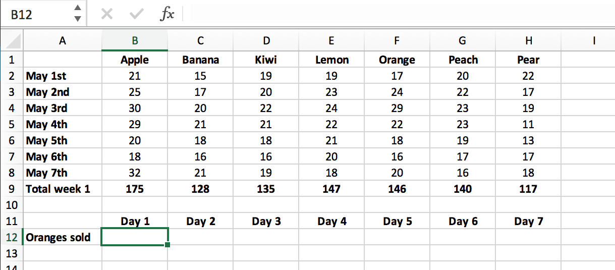
In our example we show how many pieces of fruits are sold per day in the first week of May. We want to find out how many oranges were sold each day of the week.
First, select a cell in which you want to publish the sold amount of oranges. We start with ‘Day 1’:
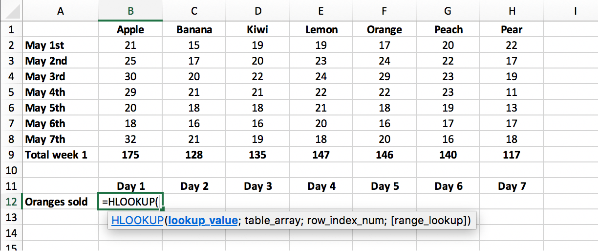
Then we select the value (from row 1) we want to look up, in this case it’s ‘Orange’ in cell F1.
We can insert this value as a string: “Orange” (image 1), or as a cell reference: F1 (image 2):
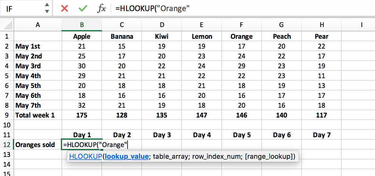 Image 1, Value as a String
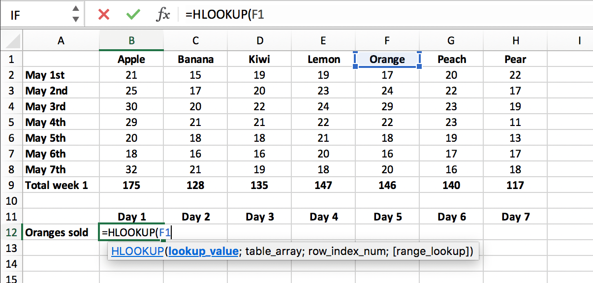 Image 2, Value as a Cell Reference
Next we enter ‘;’ and select the range (or table array) in which we want to find the lookup value and the return value. In this case it is range (B1:H8):
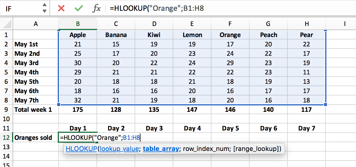
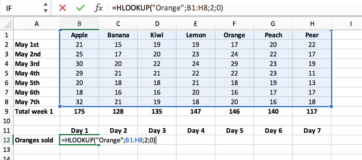
Then we enter ‘;’ and the number of the row within the defined range in which we want to look for the return value. In this case it is row 2 (for day 1), followed by ‘;’ and ‘0’ or ‘FALSE for an exact match with the lookup value ‘Orange’:
When we press enter, we get the amount of oranges sold on day 1:
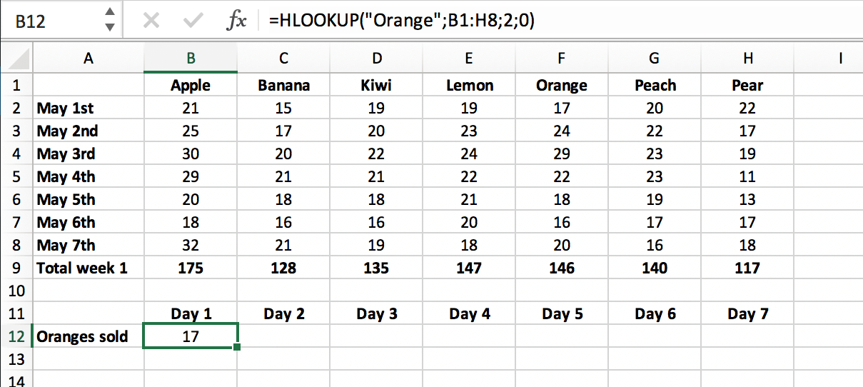
To look up the value for day 2, we can copy the HLOOKUP formula, and replace row 2 with row 3:
=HLOOKUP(“Orange”;B1:H8;3;0):
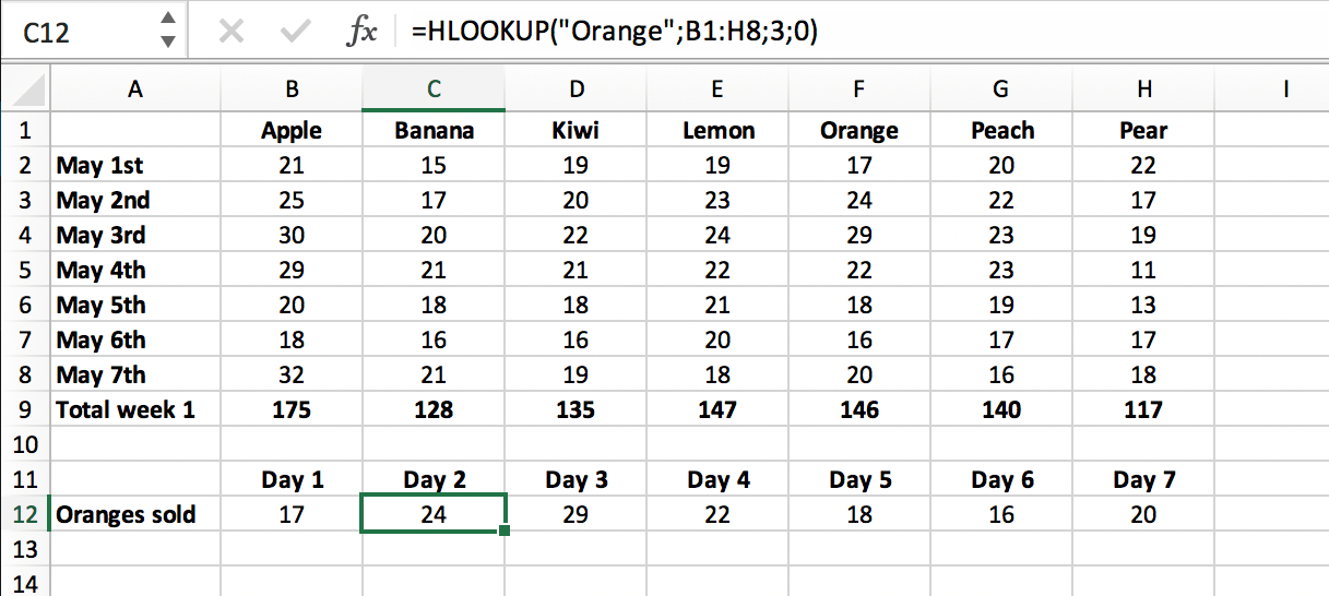
We can repeat this proces for each formula within the formula range B12:H12.
In this example we only have a small list of dates, but imagine you have a long list that publishes several years and you wish to use a certain value in other worksheets! Using HLOOKUP (and VLOOKUP) the user only has to change a certain value in one worksheet and it will automatically be changed in all other relevant places.
But what if you’re not certain about your lookup value? Then you can consider an approximate match (set False to True).
Approximate match
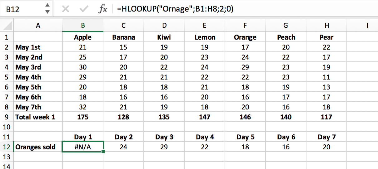
When we enter the word ‘Ornage’ in our HLOOKUP function, because we are not sure about the spelling of the value that we’re looking for. The formula as we designed it gets confused, because it can’t find this value in the table array. It returns the standard Excel error #N/A:
Let us change the ‘0’ (or ‘False’) component of our HLOOKUP function to ‘1’ or ‘TRUE’:
=HLOOKUP(“Ornage”;B1:H8;2;1)
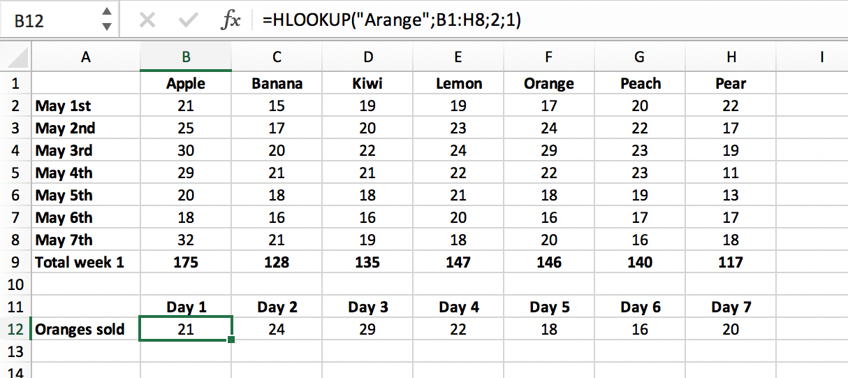
Now we have asked the function to look for an approximate match with ‘Ornage’. If it can’t find the exact match, it will look for the closest match to the value ‘Ornage’, less than ‘Ornage’, which is ‘Orange’:
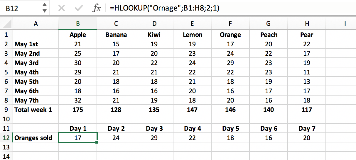
Would we enter ‘Arange’ in stead of “Orange”, the function returns 21, because then ‘Apple’ is the closest match less than ‘Orange’ (based on alphabetic order):
