Categories
How to use VLOOKUP in Excel
VLOOKUP is a function that makes Excel search for a certain value in a column (the so called ‘table array’), in order to return a value from a different column in the same row. VLOOKUP is an abbreviation for ‘Vertical Lookup’. This article will teach you how to use the VLOOKUP function.
About the VLOOKUP function
A VLOOKUP function exists of 4 components:
- The value you want to look up;
- The range in which you want to find the value and the return value;
- The number of the column within your defined range, that contains the return value;
- 0 or FALSE for an exact match with the value your are looking for; 1 or TRUE for an approximate match.
Syntax: VLOOKUP([value], [range], [column number], [false or true])
VLOOKUP example
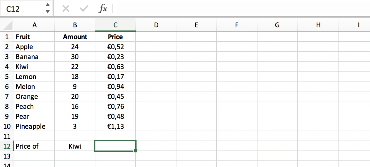
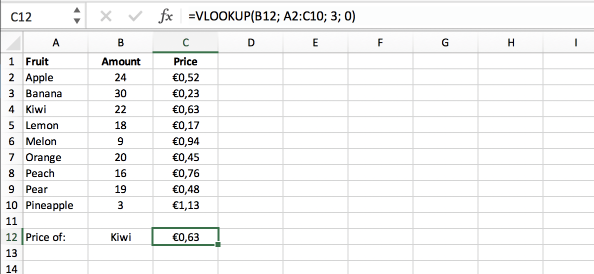
In our example we have a list of fruits, the amount in stock and the current price. We want to find the price of kiwi’s quickly in this table.
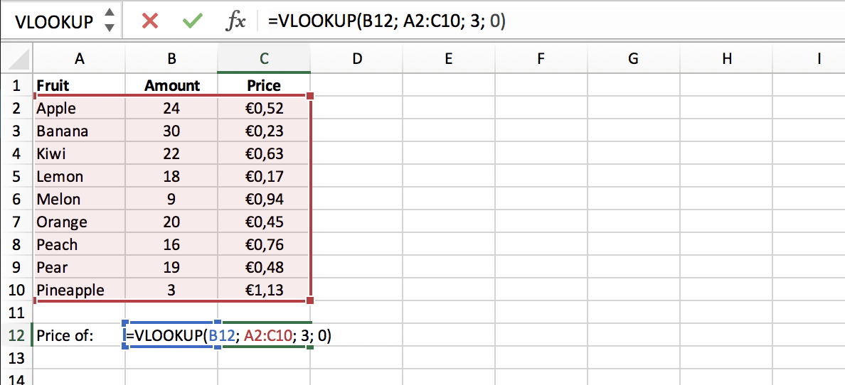
First, select a cell in which you want to publish the current price:
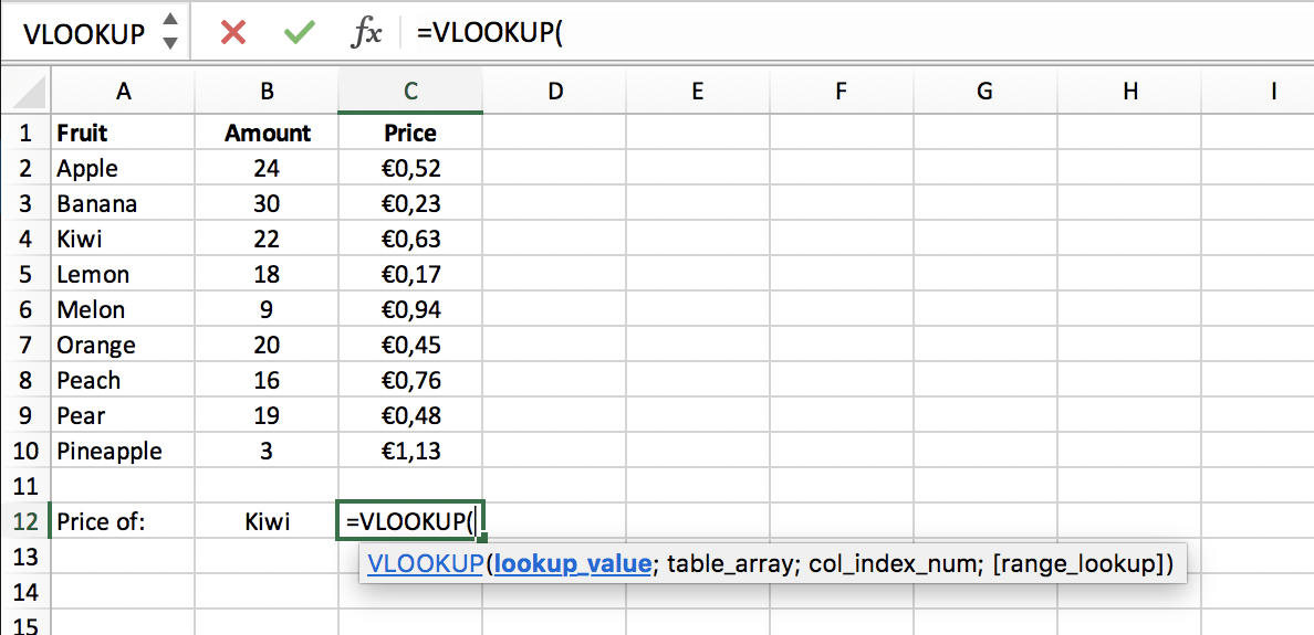
So, in our selected cell we start typing: =VLOOKUP( :
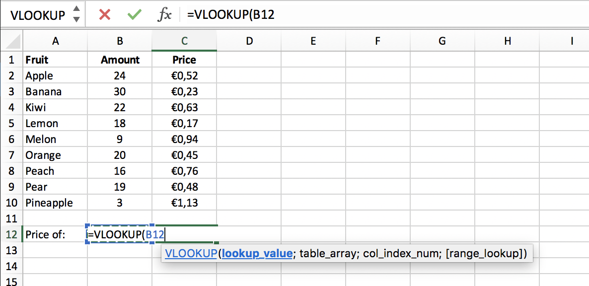
Then we select the value we want to look up, in this case it’s ‘Kiwi’ in cell B12:
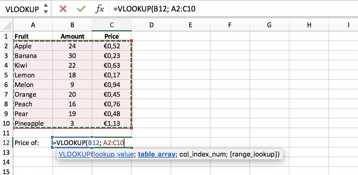
Next we enter ‘;’ and select the cell range (or table array) in which we want to find the lookup value and the return value. In this case it is range (A2:C10):
Then we enter ‘;’ and the number of the column within the defined range in which we want to look for the return value. In this case it is column 3, followed by ‘;’ and ‘0’ or ‘FALSE’ for an exact match with the lookup value ‘Kiwi’:
When we press enter, we get the corresponding price from the row that contains value ‘Kiwi’ within the selected table array:
In this example we only have a short list of fruits, but imagine having a long list of data. When you wish to use a certain value elsewhere in your spreadsheet, functions like VLOOKUP and HLOOKUP will make your life a lot easier. You will only need to change a certain value in one worksheet and it will automatically be adjusted in all other relevant places.
But what if we’re not certain about the lookup value? This is when the approximate match might be useful.
Approximate match in VLOOKUP
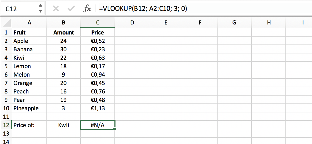
When we enter the word ‘Kwii’ in our lookup value cell B12, the VLOOKUP function as we designed it gets confused, because it can’t find this value in the table array. It will return the standard Excel error #N/A:
But we can change the ‘0’ (or ‘False’) component of our VLOOKUP function to ‘1’ or ‘TRUE’:
=VLOOKUP(B12; A2:C10; 3; 1)
Now we have asked the function to look for an approximate match with ‘Kwii’. If it can’t find the exact match, it will look for the closest match to the value ‘Kwii’, less than ‘Kwii’, which is ‘Kiwi’:
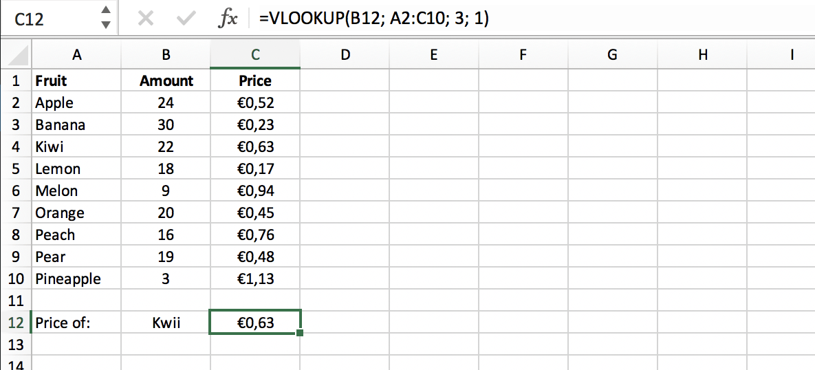
N.B. Would we enter ‘Kawi’, then ‘Banana’ becomes our closest match, because based on alphabetic order, ‘Banana’ is the first result less than ‘Kawi’. In this case the function will return €0,23.
Risks
VLOOKUP is considered a vulnerable function, since the function isn’t automatically updated when, for example, a column is added. That’s why we recommend the combination of INDEX and MATCH to get to the same results.
